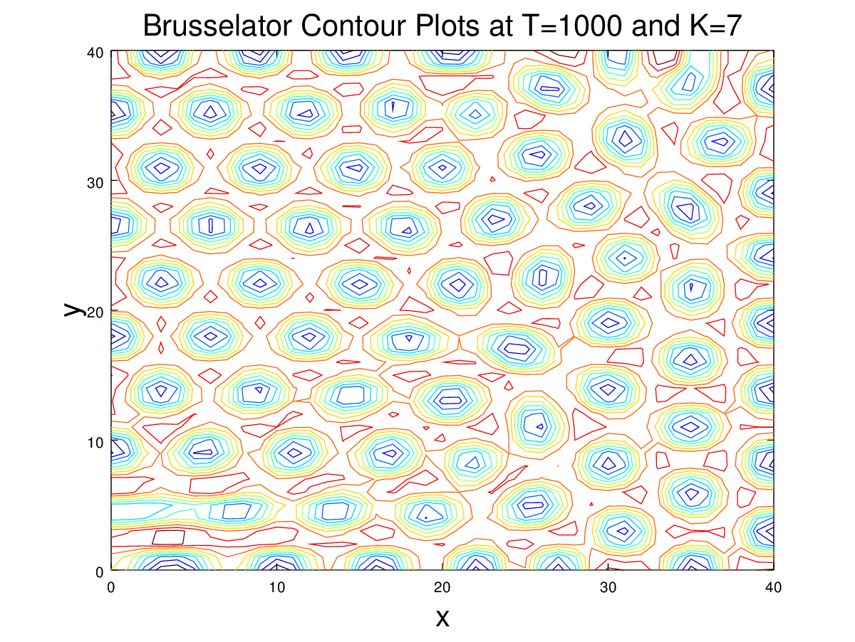
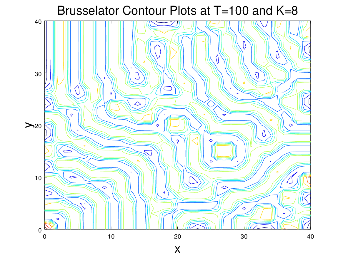
Mathematician Alan Turing proposed a possible explanation for shapes and structures found in nature. Using reaction-diffusion equations an example of emergent order in nature was seen. The patterns created are now called Turing patterns. By adding a diffusive term to a model of a stable chemical reaction, he could cause it to become unstable. This is called Turing instability and it causes a transition in which patterns evolve into a new, spatially varying steady-state solution.
An example of Turing instability is the Brusselator model. It consists of two coupled partial differential equations, each representing one species of a two species chemical reaction.
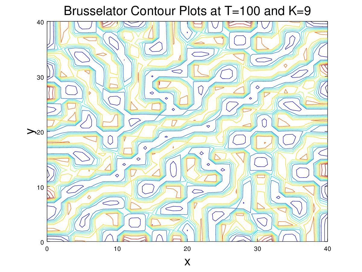
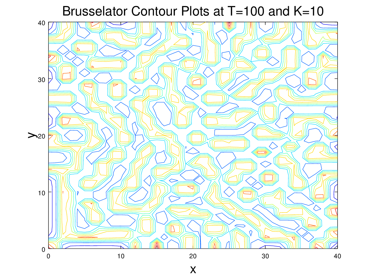
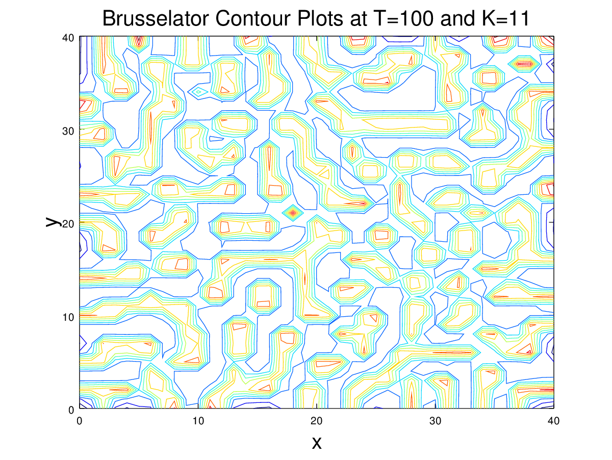
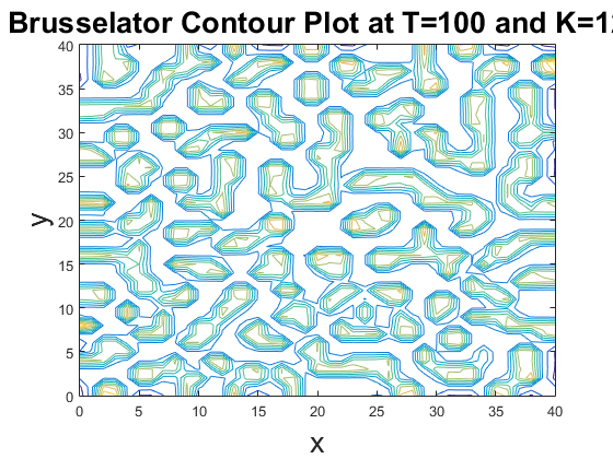
In Example 8.15 we were given two coupled partial differential equations with initial conditions and homogenous Neumann boundary conditions. The goal was to apply the Backward Difference Method with Newton's Iteration to the Brussels equations (the coupled PDEs) and reproduce the contour plots. 8.15 Code
Using the given code we were able to recreate Example 8.15. We ran the code until \(time = 1000\) for \(K = 7\) and this took well over an hour to complete. So, we only ran the other K values until \(time = 100\).


It is easily seen that with some basic algebra that the right sides of both equations will be zero.
Now we're asked the question: "For parameter settings \(Dp = 1,Dq = 8,C = 4.5\) of the Brusselator, for what values of K is the equilibrium solution \(p \equiv C,q \equiv K/C\) stable?"
We were given that a Turing instability is encountered when:
Therefore, we will have stability when:
Plugging in the appropriate values gives:
Solve the Brusselator equations for \(Dp = 1,Dq = 8,C = 4.5 \text{ and } \text{(a) } K = 4 \text{ (b) } K = 5 \text{ (c) } K = 6 \text{ (d) } K = 6.5.\) Using homogeneous Neumann boundary conditions and initial conditions \(p(x, y,0) = 1 + \cos(\pi x) \cos(\pi y), q(x, y,0) = 2 + \cos(2\pi x) \cos(2\pi y),\) estimate the least value T for which \(\lvert p(x,y,t) - C \rvert < 0.01 \text{ for all } t > T.\)
Changing the inital conditions in our code and inserting a while loop until \(\lvert p(x,y,t) - C \rvert < 0.01 \) gives: 8.4.5 Code
| K | T |
|---|---|
| 4 | 10 |
| 5 | 16 |
| 6 | 29 |
| 6.5 | 63 |
These videos of \(K = 4, 5, 6, 6.5\) are shown below on \([0,40]\times [0,40]\) with \(N = M = 40\)
Here, we went back to the original information given in the introduction of the problem, and tried to fill in the gaps between the first two figures in Example 8.15, i.e. between \(K=7\) and \(K=8\). Below are the animations on the grid \([0,20]\times [0,20]\), with \(M = N = 40\), and \(\Delta t = 1\). The code used to generate these figures is given here.
| \(K = 7.2,\; 0 \leq t \leq 100\) | \(K = 7.4,\; 0 \leq t \leq 100\) | \(K = 7.6,\; 0 \leq t \leq 100\) | \(K = 7.8,\; 0 \leq t \leq 100\) |
Because the time it took to generate these videos was very long even only going to \(t = 100\), we opted to only generate a photo for the time \(t=2000\) for these values of \(K\). Additionally, we narrowed the grid to \([0,10]\times [0,10]\), with \(N = 20, M=20\), to reduce the waiting time and still keep our grid step sizes at 0.5.
| \(K = 7.2,\; t = 2000\) | \(K = 7.4,\; t = 2000\) | \(K = 7.6,\; t = 2000\) | \(K = 7.8,\; t = 2000\) |
These results as well as the Turing instability condition formula indicate that the type of Turing pattern that is created in the Brusselator depends on the value of the K parameter. The K value needs to be larger than 6.7 to create a Turing pattern, and as can be seen at the end times of the above movies, as the K value is increased from 7 to 8, the patterns gradually change from spots to lines. In the video below, the Turing patterns for T=100 and K ranging from 6.8 to 9.8 at steps of .1 for K can be seen below. This video shows that between 6 and 10, higher K values lead to more line like Turing patterns. This video was made with this.